Friday, September 30, 2016

September 7, 2016: Propagated Uncertainty in Measurements

Anthony Betancourt
Lab Partner: N/A
Professor Wolf

Lab #6: Density and Propagated Uncertainty

Purpose: 

The Purpose of this experiment is to review the concept of significant figures and introduce the use of vernier calipers.  Also, determining the density of metal cylinders by taking measurements in order to identify the specific metal.

Procedure:

  1. Grab two different sized metal cylinders. Make sure to choose two cylinders that are of different metals.  
  2. Grab a set of Vernier Calipers. If unsure on how to use calipers be sure to watch the following video on how to use and read the vernier calipers: https://www.youtube.com/watch?v=Wo3iVrSUKPE&feature=plcp
  3. Measure each cylinder's length and width.  Keep in mind that the width will also be the diameter for the cross sectional area of the cylinder.  
  4. Measure both cylinders on electronic scales in the back of the classroom and record the masses.
  5. Once both cylinders are measured and the volume is calculated, use formula to calculate the uncertainty for your cylinders.  

Theory:  

The accuracy of your final measurement depends on the accuracy your measurement tools.  The more accurate a tool is the less amount of uncertainty there is in your final calculations.  To an extent, uncertainty will allow anyone who is verifying your calculations to determine how much a value can deviate ± for a taken measurement.  Depending on how many significant figures the readout on a measurement device is, this will determine the amount of uncertainty on a measurement.  Below is an example of a vernier caliper with a given measurement:

(Example of how to read a vernier caliper measurement)

Measured Data:

(Measurements of each cylinder)


(Formula for calculating uncertainty)

(Calculated uncertainty in iron density)

(Calculated uncertainty in Aluminum density)

Conclusion: 

The accepted masses for iron and aluminum (according to google) are 7.87 g/cm^3 and 2.70 g/cm^3.  My experimental value of iron falls within the range of uncertainty of the accepted value for the density of iron.  Also, the experimental value for aluminum is within the experimental uncertainty for the density of aluminum.  Overall, the accuracy of the measurements taken have shown to be reliable in calculating the density of metals with a low level of uncertainty.  

Thursday, September 29, 2016

September 14, 2016: Trajectories (Projectile Motion)

Anthony Betancourt
Lab Partner: Josh Fofrich
Professor Wolf

Lab #5: Trajectories

Purpose:  The purpose of this lab is to predict the impact of a projectile on an incline board with the understanding of kinematics in 2 dimensional motion.  

Procedure:  
  1. First set up the apparatus as shown on your lab table:
  2. Pick a point on the inclined V-channel to launch the ball from.  Use this launch point for each trial.  
  3. Practice launching ball off the edge of the table and notice where it lands.  Place a piece of white paper and carbon paper (carbon side down, white sheet underneath) in the area where the ball lands.
  4. Launch the ball 5 times from the same position on the ramp.  Verify that the ball lands in the same area after each launch trial.
  5. Determine the height of the bottom of the ball when it leaves the track and the distance it travels from the tables edge.  Determine launch speed of the ball from your measurements.  
  6. Place a board on an incline under the path of the balls trajectory, such that the ball will strike it when launched from the same spot.  
  7. Use smartphone to measure the incline of the board. Derive an expression that will determine the value of d along the board.  
  8. Repeat experiment 5 times launching the ball from the same spot.  
Measured Data:
(Height from where ball launches; uncertainty in ∆x; launch speed)
(expression for d along the board)
Calculated Results:
(values for calculations above; d= 0.31m; h= 0.94m ± 0.005m; V= .97m/s)

(experimental value for d)
(Theoretical value of d)


Analysis: Once the height of the ball was determined, the velocity of the ball as it leaves the track was able to be calculated from the measurements made.  The calculations are shown above in the first photo.  Once the launch speed was calculated, it was applied to the second part of the experiment where d was determined along the incline of the board.  d is the distance the ball travels before hitting the inclined board.  Calculations showing the theoretical value of d are in the last two pictures.

Conclusion:  This experiment was simple but still has inherit uncertainty in the gather-able data.  The initial height calculated has some uncertainty due the measurement is reliant on the person eye sight on where the actual bottom of the ball is in relation to the the floor.  The angle of the wooden plank might also cause skewed values due to the calibration of the smart phone elevation app.  Lastly, the theoretical expectation of d might differ from actual real world results since the calculations do not account for the ball mass as it rolls down the ramp.  The ball can travel farther down the ramp than originally calculated.

Sunday, September 25, 2016

September 12, 2016: Modeling the fall of an object with air resistance

Anthony Betancourt
Lab Partner: Josh Fofrich
Professor Wolf

Lab #4: Modeling Air Resistance
Part 1:
Purpose:  
This lab is designed to model the air resistance force on an object in free fall.  The objects being dropped in the lab are coffee filters.  The filters will fall from a height high enough to allow the filters time to reach a terminal velocity.  This velocity can be translated into data points on a position vs. time graph.  Once the position vs. time graph is plotted, the linear portion of the graph is used to calculate the slope of the line which gives us the experimental value for terminal velocity.  5 trials will be conducted in order to have sufficient data points for determining the air resistance force.   

Procedure:  
  1. Head to building 13 (Design and Technology) lobby are on the north side of the building.  The balcony is where the filters will be dropped. 
  2. Have your lab partner sit at the bottom flight of stairs set up with a video recording device.  
  3. For the first trial, 1 coffee filter will be dropped from the balcony against a black background with a meter stick attached in order to have a reference point for distance traveled by the filter.  
  4. Once the filter is dropped, the person sitting at the bottom of the stairs should start recording the free fall of the coffee filter.  Be sure to record from the same spot for each trial.  
  5. For trial 2 another coffee filter will be added to the drop.  In theory, the mass will be doubled and each consecutive trial afterwards will have an increase in mass from each filter added.  
  6. Repeat procedure until 5 sufficient trials are completed.  
Theory: 
In order to derive a value for air resistance, we model this value using the power law. evaluating the shape of the object, we can conclude that the velocity of the object directly correlates with the air resistance force it experiences.

Measured Data:

(2 coffee filters; data points from trial 2 video)
(1 coffee filter; data points from trial 1 video)
(5 coffee filters; data points from trial 5)

(1 coffee filter; position vs. time graph; slope equals terminal velocity)
2 coffee filters; position vs. time graph; slope equals terminal velocity)
(3 coffee filters; data points from trial 3 video)
(trial 3 position vs. time graph; slope equals terminal velocity)
(4 coffee filters; data points from trial 4 video)

(trial 4 position vs. time graph; slope equals terminal velocity)
(trial 5 position vs. time graph; slope equals terminal velocity)
(All five trials; Air Resistance on y-axis, terminal speed on x-axis)
 Analysis: 
The correlation of all 5 trials trials was approximately 0.96. So, trials 2 and 5 were outside the power fit curve and were not accounted in final power fit curve equation.  The values for k and n are in the text box as letters A and B, respectively, in y=A*x^B equation.  Uncertainties in k value is + or - 0.001330, uncertainties in n value is + or - 0.4563.  

Part 2:
(1 coffee filter plugged into excel model equation)
Conclusion:
After plugging in the different masses for coffee filters into the excel model, the outcome of each terminal velocity was close to the experimental outcome.  This model supports the experimental data collected and could be a useful tool in assessing any equivalent data on determining terminal velocity.  Issues dealing with trials 2 and 5 (not included in power fit curve) may have stemmed from the data points collected in the video trials.  The background on the hanging cloth was also not entirely opaque, making it difficult to get accurate data points during free fall.  One way to combat this would be to perform the experiment against a tall wall with a larger measuring stick along the wall.  Also, a video with more steady of picture to help alleviate any shakiness in recording.  

Saturday, September 24, 2016

September 7, 2016: Non-Constant Acceleration Activity

Anthony Betancourt
Lab Partner: Josh Fofrich
Professor Wolf

Lab #3: Non-Constant Acceleration

Purpose: 
The purpose of this activity is to utilize Excel in achieving a numerical approach to solving  non-constant acceleration problems.  Analytical approaches to problem solving can be time consuming and messy, therefore, plugging values into Excel can calculate large amounts of data quicker and more efficiently.  We are giving a problem of an elephant with a rocket strapped to its back, headed down a ramp at a given velocity.  The moment the elephant reaches the level surface at the bottom of the ramp, the rocket ignites and begins to thrust in the opposite direction that the elephant is traveling.  We need to find out how far the elephant travels before coming to rest.  

Procedure:
  1. Open up a new Excel spreadsheet
  2. Fill out the correct values for Vo and Xo
  3. Set delta t to be 1 second. Put in the other values in cells B1 through B4
  4. Input a formula into cell A9 that can calculate time, and fill down.  
  5. Enter an acceleration formula into B8 that will calculate acceleration at any given time.  
  6. Cell C9 enter formula to calculate the acceleration for the first interval of time.  
  7. Cell D9 enter formula to calculate change in velocity
  8. Cell E9 enter formula to calculate the speed at the end of the time interval.
  9. Cell F9 enter formula to calculate the average speed at the time interval
  10. Cell G9 enter formula to calculate the change in position at that time interval
  11. Cell H9 enter formula to calculate the position of the elephant. if done correctly you should be able to fill down contents of row 9 and see at what distance the elephant comes to rest at.  Answers should agree closely with what you solve analytically.
  12. Change time interval from 1s to 0.1s and take note of any difference made.
  13. change time interval from 0.1s to 0.05s and take note of any differences.  
Theory: 
The use of Excel provides us a way to numerically represent each second of the elephants movement until it reaches a resting point.  In order to verify our analytical method, it would be easy to double check by plugging in values generated by the spreadsheet.  In cases where it is time consuming or not possible to be performed analytically, Excel is a powerful tool that can be used to make light work of repetitive data plugging.  

Measured Data:
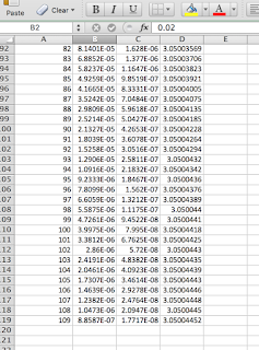
(Excel table filled out with given values from procedure)

(1 second intervals; H28 shows distance traveled before coming to rest)

(0.1 second intervals; H205 shows distance traveled before coming to rest)

(0.05 second intervals; H402 shows distance traveled before coming to rest)

Analysis:  
The Excel tables above depict the distant the elephant traveled until coming to rest in increments of 1 second, 0.1 second, and 0.05 second intervals. In order to properly depict the data, certain equations must be enter into the appropriate cells.  Cell C9 is "=(B8+B9)/2", D9 is "=((C9*$B$4))", E9 is "=(E8+D9)", F9 is "=(E9+E10)/2", G9 is "=F9*$B$4", and H9 is "=H8+G9".  As the time interval decreases, the more precise the value for the distance becomes. 
Conclusions:    
  1. Analytical results are dependent on your calculus skill and the amount of time it takes to solve the problem, Whereas, numerically solving the problem using Excel can decrease the amount of time and the likelihood of systematic errors.  
  2. Choosing the appropriate time interval to show the correct integration result depends on how exact of a value needed for the distance traveled, the small the interval the more exact of a value for delta x.  Excel is beneficial in this instance because the data table can be adjusted to calculate smaller and smaller values for time and result in a more accurate value for the distance.  
  3.   The elephant would travel approximately 164.036268 meters before coming to rest.  

Thursday, September 22, 2016

August 31, 2016: Free Fall Lab; Determination of g and Analyzing data


Anthony Betancourt
Lab Partner: Josh Fofrich
Professor Wolf
Lab Performed: 08/31/2016
Free Fall Lab

Part 1

Purpose: This experiment is to demonstrate a free falling object, determining the value of g, and to study the motion with the aid of an apparatus. 

Procedure
1.     Pull a piece of the conductive tape through the bottom of the apparatus all the way top keeping the paper “tight” with the weighted clip. 
2.     Turn on power supply to electromagnet.  Use caution once apparatus is energized and do not touch any energized parts. 
3.     Prepare wooden/metal cylinder for free fall by placing it under the electromagnet near top of apparatus so it hangs. 
4.     Turn on power to the spark generator.
5.     Hold down sparker switch on spark generator (generator sparks at 60 Hz leaving a dot on the paper as it falls).
6.     While holding down the sparker button turn off the power source for the electromagnet.  Cylinder will fall once power is turned off to electromagnet. 
7.     Turn off power to the spark generator. 
8.     Tear off paper strip and place on table top alongside a meter stick.  Place the 0-cm mark on a dot and record the position of each dot measured from the 0-cm mark. 
9.     Once each dot is measured, open up Microsoft Excel and input measured values and create a graph with trend line including R-value and equation of the line. 

Theory
Utilizing the measured points on the tape, which account for each second of free fall for the wooden cylinder, an Excel spreadsheet can be made.  Once a reasonable number of data point are uploaded into Excel, the scatter plot of data can be used to obtain a trend line and consequently derive the theoretical value of g. 

Measured Data
Graphs

(graph comparing mid-interval time with mid-interval speed)
(graph comparing distance and time)
Analysis

1.     The velocity in the middle of a time interval is the same as the average velocity for that same time interval.  For example, the time interval from 0.017 second to 0.050 seconds:
o  
o   Equation from speed vs. Time graph trend line:
2.     Acceleration due to gravity can be calculated by finding the area under the graph for speed vs. time.
3.     In order to find the acceleration using a position vs. time graph, you must pick a point on the curve and find the 1st derivative in order to find the velocity.  Then you take the second derivative of the function to find the acceleration at that point.

Conclusion
            Given the relative accuracy of this experiment, the systematic errors in the procedures hinder from obtaining a more precise value of g.  These defects could be resultant of poor measuring equipment, no taking into account any air resistance from the object falling, any friction from the cylinder making contact with the apparatus, and also the amount of data points entered into the spread sheet. 
·     
The experimental value of g should be within 10% of the accepted value.  Luckily, the measurements taken along with the number of data points that were recorded in the spreadsheet were able to establish a good amount of data for the trend line graph.  The more data points input into the computer, the more accurate the experimental value of g will be.  Along with more data points also utilizing more precise measuring equipment can lead to greater accuracy.

Part 2: Errors and Uncertainty
           

1.     Every lab group’s value of g differed with one being well below the accepted value.  Most of the experimental values were just under the accepted value except one being the actual accepted value. Subsequently, finding the exact value of g will vary from group to group because one group might have more or less data point collected from the tape measurements. 
2.     Our group’s value of g ended up being the exact same as the accepted value. 
3.     Most of the class’s values were under the accepted value for g. 
4.     Our value might differ from the rest of the class due to the amount of data points we input into the excel spreadsheet, the accuracy of the measurements taken from the tape, or also accuracy of the apparatus.  Systematic errors involved in the use of measurement instruments, equipment usage, and amount of data collected.  Random errors being those that occur when human interaction occurs, such as the actual measuring of the tape, and calculating uncertainty with the class averages. 

5.     This lab focused on the ability for individuals to work with others and run an experiment together in a timely manner with the ultimate goal of proving one method of obtaining an experimental value of g.  Some key ideas focus on data acquisition and making use of the measuring tools available to you.  Also, the use of standard deviation in calculating how replicable an experiment is to derive an expected value.  One lesson learned is the proper method of formally writing lab reports and documenting data to prove your result.